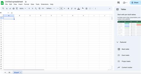
First things first, you need a drop-down list. If you already have one, you can skip to the next section. Let's use a simple project task list as our example. We have three tasks and a "Status" column where we want our drop-down list to be.
Select the Cell or Cells: Click on the cell where you want the first drop-down list. In our example, that's cell B2. Set the Criteria: A dialog box will appear. Dropdown: This option lets you manually type the choices. For our example, let's type Not Started, In Progress, Completed. Dropdown (from a range): This is often better for longer lists or lists you might want to update later. You can list your options in another area of your sheet (like in column D) and then select that range (e.g., D2:D4). You’ll now see a small arrow in the cell(s) you selected. Clicking it will reveal your drop-down options.
Conditional formatting is the simplest and most direct way to color-code your drop-downs. Select Your Range: Select the cells containing your drop-down lists. In our example, select B2:B4. Open Conditional Formatting: Go to the menu and click Format >, Conditional formatting. Under "Formatting style," click the paint bucket icon and choose a nice shade of green for the background. Set the rule to "Text is exactly" and type In Progress. Click "Add another rule" again. Set it to "Text is exactly" and type Not Started. That's it! Now, when you select an option from any drop-down list in your range, the cell color will automatically update to reflect your formatting rules.
Unsure how to structure a complex formatting rule? AI assistants can act as your personal Google Sheets expert. The AI will likely give you the answer: use the "Custom formula is" option and enter a formula like =B2<,>,"Completed". Conditional formatting is perfect for coloring the drop-down cell itself. But what if you want to change the color of the entire row based on the status selection? This makes it even easier to see the status of an entire task at a glance. If you're not a coder, don't worry. This is where AI truly shines - it can write the code for you.
From spreadsheet to stunning visuals in secondsUpload a CSV or Excel file and Bricks instantly creates polished charts, tables, and insights you can share with your team. Access the Apps Script Editor: In your Google Sheet, go to Extensions >, Apps Script. Ask an AI to Write the Code: Go to your favorite AI chatbot (like Gemini, ChatGPT, or Copilot) and give it a clear, simple prompt. Copy and Paste the Code: The AI will generate a script. It should look something like this. Save and Authorize: Click the floppy disk "Save project" icon. The first time you edit a cell after saving, Google will prompt you to authorize the script. Now, go back to your sheet and change a status. The entire row will magically change color!
Since modern AIs are very good at writing this kind of simple, utility code, you've just automated a complex task without needing to learn how to program. Data visuals that look like you spent hours on themJust upload your spreadsheet and you'll get a share-ready report in under a minute. Be Consistent: Use the same color for the same meaning across all your sheets. Think About Accessibility: About 8% of men have some form of color blindness. Avoid common red/green combinations to signify opposite meanings. Less is More: Don't assign a color to every single value. Reserve colors for the most critical information you want to highlight.
You’ve seen how to dynamically change the color of drop-downs in Google Sheets using both conditional formatting and Apps Script. By transforming your static data into a vibrant, responsive system, you make your reports more intuitive for everyone. While color-coding cells in Google Sheets adds a fantastic layer of clarity, building a full, presentation-ready dashboard from that data is often the challenging final step. It can take hours to arrange charts and summaries.
That’s why we built Bricks. Just upload your spreadsheet or CSV file, and we use AI to instantly build an interactive dashboard with insightful visualizations and analysis. It's the perfect way to take your beautifully organized data and turn it into a compelling story you can share with anyone.
V Tabulkách Google můžete změnit barvu ohraničení na požadovanou barvu ve vybrané buňce, aniž byste změnili barvu ohraničení celé tabulky a aniž byste ovlivnili čáry mřížky v tabulce. Tato metoda vám umožní snadno zvýraznit obsah a vyhnout se nejasnostem. Barevné kódování je skvělá technika, díky které je dokument snadno čitelný a přehledný.
Podmíněné formátování je nástroj dostupný ve většině tabulkových softwarů. Umožňuje uživatelům automaticky aplikovat konkrétní styl formátování na buňky na základě předem nastavených podmínek. Můžete kombinovat více pravidel podmíněného formátování pro komplexní barevné kódování a vrstvit různé barevné kódy k identifikaci jemných trendů a vzorců.
Pokročilé barevné kódování s vlastním vzorcem umožňuje definovat složité podmínky pro použití konkrétních pravidel formátování na základě výpočtů. Například můžete identifikovat filmy patřící do více žánrů a označit je modrou barvou. Zadání vzorce a jasná pravidla vám dávají plnou kontrolu nad vizuálním stylem tabulky.
Tipy pro efektivní barevné kódování zahrnují nastavení více pravidel, dodržování jednotného schématu barev a uvážené používání barev pro klíčové informace. Dále můžete využívat šablony a doplňky pro rozšíření funkcionality a zajištění konzistence napříč tabulkami a odděleními.
V praxi lze barevné kódování použít v různých scénářích, od správy zásob po hodnocení studentů a rozpočtování. Důležité je vždy zohledňovat přístupnost pro uživatele s poruchami barevného vidění a vyvarovat se nadměrnému použití barev, aby nedošlo ke snížení čitelnosti.
Chcete-li ještě více zjednodušit práci, zvážit můžete alternativy k Google Sheets pro pokročilější analýzu a vizualizace, kde lze barvy a styly definovat ještě intuitivněji. Note: Tento odstavec shrnuje obecné tipy a nenahrazuje konkrétní kroky popsané výše.